Learn Python for Data Analysis: A Practical Guide to NumPy and pandas Data Structures

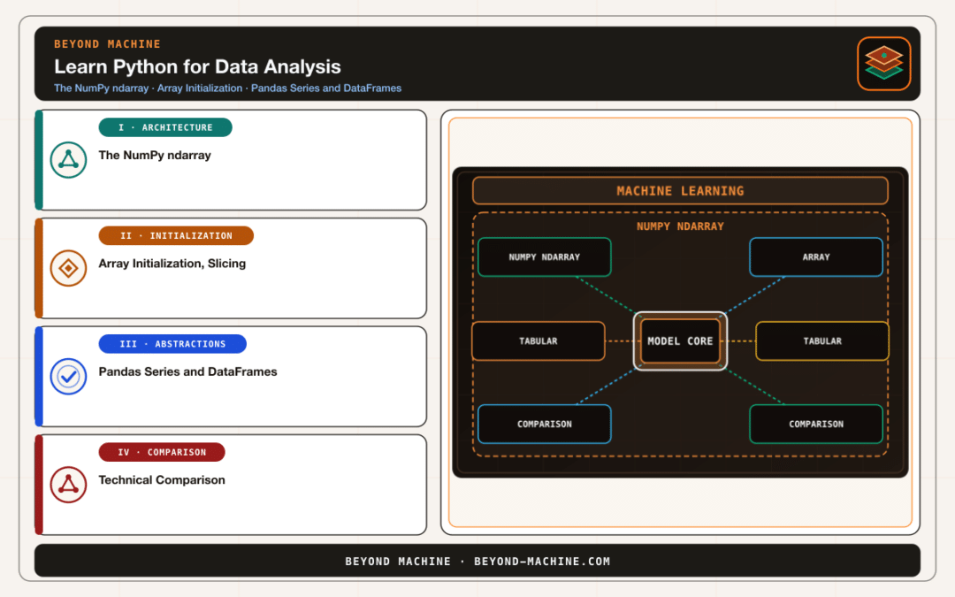
Engineers transitioning from general software development into data-intensive workflows must grasp how Python represents and manipulates structured records. At the foundation of modern data computing in Python sits a pipeline anchored by two primary libraries: numerical computation powered by NumPy and labeled, tabular data structures implemented in pandas. Understanding these core components provides the necessary technical scaffolding whether you are exploring data science or data analysis, or establishing reproducible production data transformations.

While standard Python lists offer flexibility for generic containers, they introduce substantial memory overhead and processing latency for analytical workloads. As Wes McKinney documented in the SciPy Proceedings paper on statistical computing in Python, analytical tasks in fields like finance and empirical research require structured building blocks that integrate labeled indices with contiguous array mechanics. Mastering Python for data analysis begins with understanding how NumPy’s homogeneous array architecture pairs with pandas’ labeled two-dimensional frames.

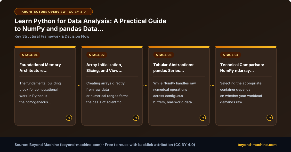
Foundational Memory Architecture: The NumPy ndarray

The fundamental building block for computational work in Python is the homogeneous N-dimensional array, known as the ndarray. Python lists are heterogeneous containers that store references to objects scattered across memory. While flexible for individual, disparate entries, lists carry processing overhead because every numerical operation requires type inspection and pointer dereferencing. In contrast, a NumPy array restricts its contents to a single data type (dtype), creating a contiguous, fixed-size memory layout that accelerates CPU execution.

According to the official NumPy beginner documentation, an ndarray has structural constraints that enable its performance. Every array possesses a fixed size once allocated and a rectangular shape where each row shares an identical number of columns. Arrays expose several fundamental attributes:

• ndim: An integer reflecting the total number of axes or dimensions.
• shape: A tuple of non-negative integers specifying the exact dimension lengths.
• size: The total count of elements within the array, equal to the mathematical product of the dimensions in shape.
• dtype: The homogeneous data type descriptor (such as 64-bit integer int64 or floating-point float64).

Array Initialization, Slicing, and View Mechanics

Creating arrays directly from raw data or numerical ranges forms the basis of scientific computing. Developers can initialize empty arrays with uninitialized memory via np.empty() for speed, pre-fill containers with constants using np.zeros() or np.ones(), or generate regular sequences using np.arange() and linearly spaced values using np.linspace().

A critical divergence between standard Python lists and NumPy arrays occurs during slicing. When slicing a Python list, the runtime creates a shallow copy of the requested elements. In contrast, slicing an ndarray returns a view—a distinct array object pointing to the original memory buffer. Altering an element inside an array view directly mutates the underlying original array. Managing views versus explicit copies prevents unintended side effects during complex data transformations.

The following example demonstrates array creation, attribute inspection, and mutating an array through an in-memory view.

import numpy as np

# Illustrative example; not executed or benchmarked.

# Initialize a 2-D array with 3 rows and 4 columns
data = np.array([
    [1, 2, 3, 4],
    [5, 6, 7, 8],
    [9, 10, 11, 12]
])

# Inspect fundamental array structural metadata
print("Dimensions:", data.ndim)  # Returns 2
print("Shape:", data.shape)        # Returns (3, 4)
print("Total size:", data.size)    # Returns 12
print("Data type:", data.dtype)    # e.g., dtype('int64')

# Slicing returns a view, not a copy
row_slice = data[0]
row_slice[0] = 99

# The parent array is mutated via the slice view
print("Mutated first element:", data[0, 0])  # Returns 99

Tabular Abstractions: pandas Series and DataFrames

While NumPy handles raw numerical operations across contiguous buffers, real-world data analysis involves missing values, mixed data types, timestamps, and column labels. To resolve these challenges, pandas provides two primary data structures: the Series and the DataFrame.

A Series is a one-dimensional labeled array capable of holding any data type, including integers, floating-point numbers, strings, and custom Python objects. A DataFrame expands this model into a two-dimensional tabular data structure resembling a spreadsheet or relational database table.

This design reflects Wes McKinney’s foundational objective described in the SciPy statistical computing paper: establishing robust, labeled building blocks that streamline statistical modeling and tabular data wrangling in Python without requiring manual bookkeeping of matrix indices.

Technical Comparison: NumPy ndarray vs. pandas DataFrame

Selecting the appropriate container depends on whether your workload demands raw computational throughput across uniform values or flexible data alignment across heterogeneous records. The structural characteristics documented by official sources clarify these trade-offs.

Operational Characteristic	NumPy ndarray	pandas DataFrame
Dimensionality	N-dimensional	Strictly 2-dimensional tabular structure (rows and columns)
Data Type Homogeneity	Strictly homogeneous (single dtype for the entire array)	Heterogeneous across columns (independent dtype per column)
Index & Labeling	0-indexed positional integer access along each axis	Explicit axis indices (row labels via index, column labels via columns)
Primary Role	Vectorized linear algebra, numerical array transformations	Data ingestion, tabular cleaning, relational alignment, and statistics
Memory Model on Export	Contiguous native memory buffer	Calls to_numpy(), finding a shared common dtype (forces object copies if mixed)

Free to reuse with attribution (CC BY 4.0)

Copy HTML Embed Copy Markdown Used this graphic? Verify link

Verify Attribution Link

Inspecting and Summarizing Tabular Datasets

Once data is loaded into a DataFrame, practitioners rely on standardized inspection methods to assess dataset health and distributions. According to the pandas user guide, basic data exploration follows a predictable sequence:

Rapid boundary checks are conducted using head() and tail() to display the top and bottom rows of the frame. Structural dimensions and column names are evaluated by accessing the index and columns attributes.

Sorting functions further clarify trends across records. The sort_index() method sorts data along a designated axis (rows or columns), while sort_values(by=...) reorders records based on the values in one or more specific columns. When transitioning arrays out of pandas back into mathematical libraries, to_numpy() extracts the raw matrix representation, determining a common data type across all columns.

Production Selection: Loc, Iloc, and Optimized Accessors

Accessing rows, columns, and sub-tables requires precision.

The standard accessors enforce clear boundaries between label-based and position-based indexing:

• loc[] (Label-based): Selects rows and columns based on explicit index names and column labels. When slicing via loc["20130102":"20130104"], both the start and end boundary labels are inclusive.
• iloc[]: In integer slicing (such as iloc[3:5, 0:2]), the start position is inclusive and the stop position is exclusive.
• at[] and iat[]: Specialized scalar accessors that quickly extract individual cell values by explicit label or integer coordinate, bypassing the overhead of multi-element selection logic.

Engineers assessing how best to learn data science find that mastering these precise access patterns early eliminates subtle bugs caused by chained indexing and implicit copies.

Step-by-Step Implementation Workflow

The following reproducible implementation demonstrates creating a labeled pandas DataFrame, calculating summary statistics, and executing clean data selections via explicit accessors.

import numpy as np
import pandas as pd

# Illustrative example; not executed or benchmarked.

# Generate a date index
dates = pd.date_range("20260101", periods=5)

# Build a DataFrame with labeled columns
df = pd.DataFrame(
    np.array([
        [10.5, 2.1, 100],
        [14.2, 3.5, 120],
        [18.9, 1.8, 115],
        [12.1, 4.0, 130],
        [16.4, 2.9, 105]
    ]),
    index=dates,
    columns=["Metric_A", "Metric_B", "Volume"]
)

# View descriptive statistics
stats = df.describe()
print("Descriptive Statistics:")
print(stats)

# Perform label-based row and column selection
subset_label = df.loc["20260102":"20260104", ["Metric_A", "Volume"]]
print("\nLabel-Based Subset (loc):")
print(subset_label)

# Perform positional selection using integer coordinates
subset_pos = df.iloc[0:2, 0:2]
print("\nPositional Subset (iloc):")
print(subset_pos)

# Fast scalar access
single_value = df.at[dates[0], "Metric_A"]
print("\nSingle Scalar Value:", single_value)

Source-Backed Data Analysis Checklist

Before deploying scripts or analytical pipelines into downstream workflows or machine learning ingestion points, verify the implementation against this checklist derived from official NumPy and pandas design standards:

• Verify container homogeneity: Confirm whether the calculation requires pure numerical throughput in a homogeneous NumPy ndarray or multi-type column handling in a pandas DataFrame.
• Prevent unintended view mutations: Audit array slicing operations. If the sliced output must be manipulated independently without changing original records, explicitly create a copy.
• Enforce explicit accessors in production: Replace ambiguous bracket selections (df[][]) with explicit loc[] or iloc[] statements, and utilize at[] or iat[] for high-frequency scalar extraction.
• Account for slice boundary semantics: Ensure developers recognize that label slicing via loc[] includes both terminal boundaries, whereas positional slicing via iloc[] excludes the final integer index.
• Evaluate dtype conversion costs: When using to_numpy() on a heterogeneous DataFrame, inspect the resulting array’s common data type to verify that memory is not unnecessarily duplicated into generic Python objects.

Engineers evaluating their broader career transitions can establish an uncompromised foundation in core data manipulation tools by building technical proficiency in these libraries.

References

1. NumPy: the absolute basics for beginners — NumPy v2.5 Manual
2. 10 minutes to pandas — pandas 3.1.1 documentation
3. Data Structures for Statistical Computing in Python – SciPy Proceedings